A Petri net Modeling and Simulation of Lotka-Volterra (rabbit and fox) system

Abstract

Rabbit and fox system of Lotka and Volterra has been modelled using stochastic Petri net model. The Petri net model was verified employing P-invariance as well as T-invariance. It has been concluded that with lower number of interactions between prey and predator the variations in the population of prey as well as predators follow exponential distributions which become oscillatory at higher interaction levels. For all these computations the Gillespie method of stochastic simulation (Journal of Physical Chemistry Voi. 8 1, No. 25, 1977) was followed and a computer program in matlab was used for simulations.

Keywords

Stochastic Petri net, stochastic modelling, Lotka-Volterra

Introduction

The field of Simulation and modelling is one of the fast developing areas in computer science.  Modelling is a graphical or mathematical description of elements of a system of interest. A model is better, if it can be used by a computer to simulate the behaviour of the system. It is worth mentioning that reactions and Petri nets both posses two kinds of players (reactions posses molecules and reactions and Petri nets posses places and transitions) and therefore Petri nets can be used for modelling reactions. The basic objective of modelling is the better understanding of the problem.  Modelling can also help arrive at correct mechanism of a reaction.  It also provides a cheaper way of studying a phenomenon as compared to studying the same in laboratory. The transformation from an informal to a formal model involves the resolution of any ambiguities, which must not happen necessarily in the right way. Therefore, the next step in a sound model-based technology for behaviour prediction should be devoted to model validation. Model validation aims basically at increasing our con?dence in the constructed model. It is important to go for model validation before model analysis. So, before thinking about model analysis, we are concerned with model validation.

Petri net is a directed bipartite graph suggested by Petri in 1960 [1].  Petri nets provide a range of powerful analysis and simulation techniques [2, 3, 4, and 5].  It consists of places represented by circles and transitions represented by rectangles. Places connect rectangles and rectangles connect places by edges represented by arrow and contain weights. Places contain tokens represented by dots. A transition is enabled to fire if number of tokens in each input place p of a transition is greater than or equal to weight w (p,t) of the arc  from place to transition. The firing does not take any time.   A Petri net model for the reaction 2C + O2 = 2CO is shown in Figure. 1     

Figure. 1 Petri net model for reaction 2C + O2 = 2CO

After its discovery in 1960 there have been new developments to the theory [4-8] which are briefly described below:  

1.1 Stochastic Petri nets (SPN)

Stochastic Petri nets (SPN) are developed to introduce time and probability to the system. An example of SPN is the modelling of coupled chemical reactions.  SPN are associated with an exponentially distributed firing rate to each transition. Occurrence of next reaction is decided by Gillespie algorithm.  Detail of SPN is provided in section 3.

1.2 Continuous Petri nets (CPN). In such Petri nets places are represented by double circles, transitions are represented by hollow rectangles and tokens are real numbers. Transitions possess a firing quantity which can be any quantity between 0 and m where m is the token in the input place.  A simple example of continuous Petri net is pumping of a liquid between two vessels is pictorially shown, in Figure. 2, 

Figure. 2 CPN model of pumping liquid. T1 continuous transition, P1, P2 continuous places containing real amount.

Here P1 represents the vessel 1, P2 represents vessel 2 and T1 represents the pump.  Firing quantity multiplied by the weight on the arc decides the amount of liquid withdrawn from P1 or deposited to P2. Suppose P1 contain 9.3 units of liquid and firing quantity if T1 is 3.2 and the weight on the outgoing arc is 2.0 then a quantity of 6.4 will be withdrawn from P1 and deposited to P2.

1.3 Hybrid Petri net (HPN).  Such Petri nets consist of continuous part as well as discrete part.  A simple example of HPN is pumping of a liquid from one tank to the another, operated by switches.  The tanks containing liquid are continuous parts and switches use for starting or stopping the pump are discrete parts. The system is depicted in Figure 3

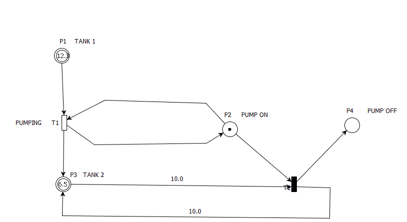
Figure. 3 HPN model of pumping liquid

 Places P1, P3 and transition T1 are continuous parts P1 contain 12.3 units of liquid and P2 contain 6.5 units of liquid and firing capacity of T1 is 0.1.  P2, P4 and transition T2 are discrete parts. P2 and P4 are switches and T2 is a discrete transition. In the current state the switch P2 contain a token and in 35 units of time pumps 8.8 units of liquid from P1 decreasing its content to 8.8 units deposit 3.5 units to P3 making it total content to 10 units. This enables T2 which consumes a token from P2 deposits to P4 and disables T1.

 1.4 Hybrid Functional Petri net (HFPN). It is an extension to HPN. It contains two additional arcs namely test arcs and inhibitory arcs, these arcs can be only input arcs. A test input arc is directed from a place of any kind to a transition of any kind. It does not consume the content of the source place.  Inhibitory arcs prevent the transition from firing if the content of the input place is greater than or equal to weight of the inhibitory arc.  The continuous transition in HFPN is similar to that used in HPN and some function can be assigned to it for firing rate. Besides these, it is also possible to assign any function (values of places) to arcs; such possibilities are helpful to model composition of tetramer in terms of monomers as shown in figure 4. V1, V2 and V3 can be functions of values of places P1 and P2.  As four monomers are needed for one tetramer V2 can be written as 4*V3.

Figure. 4 A HFPN model for composition of tetramers out of monomer.

1.5 Hybrid Functional Petri nets with extension [HFPNe] takes into account the spatial information such as position and speed of a place.  Besides using real and integer values, it is also possible to use strings (DNA sequences) and objects with variables and methods. HFPNe also use generic places (mRNA sequence, phosphorylation state of a protein) and generic transitions (complex reactions by updating the state of connected entities).  The entities used in HFPNe are shown in Figure 5.

Figure. 5 Basic entities in the HFPNe architecture

Most of the publications [9-16] on prey and predators   are based on   first order non-linear ordinary differential equations (ODE). There is one ODE for each variable.  Equations are deterministic and single valued.  These equations can be written as:

dx/dt  =   c₁ x  - c₂ xy                              1

dy/dt  = c₃ xy -  c₄ y                                2   

Where x and y are the number of prey and predators respectively.  Equations 1 and 2 represent the instantaneous rates of the prey and predators respectively at time t.  c₁, c₂, c₃ and c₄ are positive real constants.  Equation 1 shows the rate of production (c₁ x) and death (c₂ xy) of prey. Obviously, rate of production depends only on the population of prey and   rate of death depends on the population of prey as well as predators.  Equation 2 represents the growth rate of predators which is proportional to the interaction between prey and predators minus rate of natural death of predators. At equilibrium    

           Y =c1c2

                             3                                                                                              

            X= c3c4

                             4

Equation 3 implies that at equilibrium population of predators depends upon prey parameters.  Thus increasing prey parameter c₁ will help increase predator population.

The uses of deterministic techniques such as ODEs apply to macroscopic systems and rely on a number of assumptions such as   concentrations,   are well defined, vary deterministically and continuously over time. Rate constants are also well defined. However, the approach may not apply well to the microscopic systems.

2. Petri net invariants and conservation rules.

Although Petri net graph is self explanatory, the graph alone is not enough to explain its  mathematical properties  such as  place invariant (p-invariant) [7, 8] and transition invariant (t-invariant). Both concepts are derived from mathematics. Presence of invariants confirms the correctness of the net. Invariants in Petri net indicate states that do not alter after a transformation or a sequence of transformations.  A place vector is called P-invariant if it is solution of the linear equation system.

           X.C=0                            2.3

   Here C called incident matrix of the net and is given by C = [aij] n x m, where n is the number of places and m is the number of transitions, rows correspond to places while columns correspond to transitions.  Every entry aij, is an integer number equal to a difference between the numbers of tokens in place pi after and before firing transition tj. X should be positive integer and should be > zero

 Similarly, a transition vector is called T-invariant if it is a solution of the linear equations system 

      C.Y=0.                             2.4

       Y holds a positive integer > 0   

Properties of P-invariants:

(a) Number of X vectors equals number of places in the net.

(b) Non-zero elements of X vector are called support of P-invariants.

(c) If there is more than one P-invariant then support of one P-invariant should not be sub-set of any other support.

(d) A net is covered by P-invariants if every place belongs to some P-invariants.

(e) If greatest divisor of the non zero elements is 1 then P-invariants are minimal.

Properties of T-invariants:

(a) Number of Y vectors equal number of transitions in the net.

(b) Non-zero elements of Y vectors are called support of T-invariants.

(c) If greatest divisor of the T-invariant is 1, then the variant is minimal.

(d) All invariance computations were made employing PIPE (platform independent Petri net editor) program. Let us consider the net shown in Figure. 6 for the incident matrix is:

                 1-1         00   1    -1

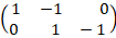
Place vectors are:

                    X=(x₁, x₂)

P-invariants are solution of equation X.C=0

                    Or

                    x1x21-1         00   1    -1

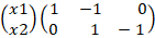
  =0

The net is not covered by positive P- invariants therefore it does not seem to be bounded.

(e) T-invariants are solution of the equations C.Y=0.  Since the net passage 3 transitions there will be three components of Y says Y₁, Y₂ and Y₃. For obtaining T-invariants we need to solve the system.

                   1-1         00   1    -1. Y 1Y2Y3

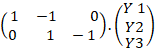
= 0

We obtained following one solution

                             T1    T2   T3

T-invariant 1         1       1      1   

Which suggest that the net is covered by T-invariant and is supposed to be bounded and live.

Figure. 6  Petri net model for rabbit and fox

3. Stochastic Petri net and simulation

SPN can be defined as N = (P, R, Pre, Post, h, X), Here P is the set of places, R the set of transitions, Pre is the multiplicities of place-transition edges, Post gives the multiplicities of transition-place edges and h is the probability rates function. In SPN transitions can be either timed or immediate.   While timed transitions are associated with exponential distribution of firing delays firing of immediate transitions consume no time.   In the present paper we are concerned the simple SPN with time transitions. Such SPN are applicable to those reactions which operate in an unco-ordinated, asynchronous way, and the reaction events happen at exponential random times. Simulation of such reactions can be performed with the help of Gillespie algorithm.  Suppose there are v reactions in a given coupled reaction system, hazard for a type i reaction is h_i(x,c_i), and the hazard for the whole reaction h₀(x,c) is 1v hi(x,ci)

.  Also the time to next reaction is EXP (h₀(x,c)) and the reaction type will be i with probability h_i(x,c_i)/h₀(x,c).  Thus the Gillespie method provides a method for computing the time and type of next reaction enabling to compute the state of the system.

The present problem of rabbit and fox as prey and predator was undertaken with the objective of treating it as a discrete and stochastic problem instead of as a continuous problem as undertaken by many others [9-16].  For this purpose, Petri net was chosen as a suitable model.  The Petri net model is shown in Figure.6.  P1 and P2 denote the prey and predator places respectively and R1, R2 and R3 represent the transitions. Arcs join places to transitions and vice versa. Arcs have capacity 1 by default; if other than 1, the capacity is marked on the arcs. Transition R₁ represents the growth of prey utilizing resources. R₂ represents the interaction of prey and predators, death of prey and increase in population of predators. Ultimately R₃ represents death of predators. In the present simulation we define these 2 by 3 matrices namely M_pr, M_po and M. M_pr is the matrix of place to transition multiplicities, Mpo is the matrix of transition to place multiplicities and M = Mpo – Mpr is the stoichiometric matrix. It is worth mentioning that there are two places and three transitions. Each row in the matrix is separated by a semi colon.  Thus

  M_pr = [1 1 0; 0 1 1]; M_po = [2 0 0; 0 2 0]; N is the maximum number of reaction steps.

The Lotka-Volterra ecological equation can be written as:                               

                             A  à   2A

                             A + B   -> 2B

                                   B   -> 0

Here A and B represent prey and predators respectively.  The first equation represents growth of prey species. The second equation represents interaction of prey and predator and growth of predators.  The third equation represents   death of predators.  C_1, C₂ and C₃ are reaction constants.

Let the initial value of the state vector X = X₀ .Additional data needed for such calculations are the reaction rates, h(r, X). These are functions of the reaction r and of the state X and are calculated from the mass-action kinetics. Thus  h(r1, X )= c1 X(A),  h(r2, X )= c2 X(A)X(B) and

 h(r3, X) = C3 X (B).  Compute the total reaction hazard h0 (X, C) = 1v hi(X,ci)

  for the reaction.  The time for the next reaction was computed using the relation t’ = Exp (h₀ (X, C)).  Therefore total time elapsed is t = t + t’. The reaction J was computed as a discrete random quantity with probability hi (X,c_i) / h₀ (X, C).  

Computations were made with the help of a modified Matlab computer program written by Renato Feres[17] N is the maximum number of reaction steps.  In these calculations rate constants were taken to be 1.0, 0.003 and 0.4.  X values were taken to be 60 preys and 120 predators.   It was found that upto reaction steps of 800 the variations in the size of prey and predators was exponential beyond this it becomes oscillatory. This behaviour is shown in figure 7 and 8

Figure. 7 Time vs Populations of prey -predator

Figure. 8 Time vs Populations of prey -predator

Number of oscillations increased with increase in the number of reaction steps.

REFERENCES

1. C A. Petri, Communication with Automata, New York: Griffiss Air Force Base, Tech. Rep. RADC-TR., 1,165-377 (1966).
2. M.A. Marsan, G. Balbo, G. Chiola, G. Conte, S. Donatelli, and G. Franceschinis. An introduction to generalized Stochastic Petri nets. Microelectronics and Reliability, 31(4):699–725, (1991)
3. T. Murata. Petri nets - properties, analysis and applications. Proceedings of the Ieee, 77(4):541–580 (1989).
4.  D.T. Gillespie, Exact stochastic simulation of coupled chemical reactions, The Journal of Physical Chemistry   Vol. 81, No. 25, (1977)
5. Wim Bos, Modelling biological systems using Petri nets http://genome.ib.sci.yamaguchi-u.ac.jp/~pnp/ (2008-03-30)
6. J.L. Ian Wee, Y. Yang and L. Hai, Validation of Petri net apoptosis using P-Invariant analysis, In IEEE International Conference on Control and Automation, Christ Church, New Zeeland, (Dec 9-11, 2009).
7. M. Heiner and I. Koch, J Cortadilla and W. Reisig (eds), In ICATPN 2004, Springer-Verlag, Berlin Heidellerg, Petri net-based model validation in system biology, LNCS 3099:216-237, (2004).
8. I. Koch, B.H. Junker and M. Heiner, Application of Petri net based analysis techniques to signal transduction pathways, BMC  BIOINFORMATICS, 21(7) 1219–1226, (2005).
9. Reza Kusuma Nurrohman, A. Ardiansyah, Bayu Dwi Apri Nugroho,  Lotka-Volterra Model Simulation  for Rice-field Rat and Tyto Alba Owls in Sumpiuh District,Banyumas Regency, Central Java,  Agritech, 39 (4) 323-332, (2019).
10. Y. Takeuchi, N.H. Dub, N.T. Hieu, K. Satoa. Evolution of predator-prey systems described by a Lotka-Volterra equation under random environment, J. Math. Anal. Appl. 323 938–957, (2006).
11. Peter J. Wangersky. LOTKA-VOLTERRA POPULATION MODELS, Ann. Rev. Ecol.Syst. 9:189-218, (1978).Copyright (1978 by Annual Reviews Inc. All rights reserved)
12. Sundarapandian Vaidyanathan. Lotka-Volterra Two Species Competitive Biology   Models and their Ecological Monitoring, International Journal of PharmTech Research CODEN (USA): IJPRIF, ISSN: 0974-4304 Vol.8, No.6, pp 32-44, (2015)
13. Sundarapandian Vaidyanathan. Lotka-Volterra Population Biology Models with Negative Feedback and their Ecological Monitoring, International Journal of PharmTech Research CODEN (USA): IJPRIF, ISSN: 0974-4304 Vol.8, No.5, pp 974-981, (2015)
14. Guy Bunin. Ecological communities with Lotka-Volterra dynamics, PHYSICAL REVIEW E 95, 042414 (2017) Department of Physics, Technion-Israel Institute of Technology Haifa 32000, Israel (Received 23 March 2017; published 28 April 2017)
15. Chang-Hyeon Choi1,2 Generalizations of the Lotka-Volterra, Population Ecology Model: Theory, Simulation, and Applications, Nonlinear Dynamics, Psychology, and Life Sciences, Vol. 1, No. 4, (1997).
16. R. Srivastava, L. You, J. Summers and J.Yin, Stochastic vs. Deterministic Modeling of Intracellular Viral Kinetics, J. theor. Biol., 218, 309-321, (2002).
17. Renato Feres, Notes for Math 450, Stochastic Petri nets and reactions http://www.math.wustl.edu/~feres/publications.html

REFERENCES

Smita Tripathi, Mukesh Malviya, R. Prasad*, A Petri net Modeling and Simulation of Lotka-Volterra (rabbit and fox) system, Int. J. of Pharm. Sci., 2025, Vol 3, Issue 3, 591-597. https://doi.org/10.5281/zenodo.14994693
10.5281/zenodo.14994693